How to Get Consistent Classification From Inconsistent LLMs?

A technique for deterministic labeling from stochastic models, with benchmarked Golang implementation.

TLDR: If you don’t care for the entrée, you can jump directly to Results & Code section.

---

I saw a recent Reddit post where a senior ML engineer was complaining that his job has been reduced to calling APIs of the big model providers and he no longer does ML work himself anymore.

Courtesy of Gemini

In fact, Andrew Ng said during a lecture titled Opportunities in AI at Stanford (2023 is the time of recording), that it no longer makes sense to train a NLP sentiment classifier. 7 lines of code calling OpenAI’s API will get you the same or superior results in less than 5 minutes, at a reasonably low marginal cost.

One of the biggest data problems that LLMs can help us solve is labeling large amounts of unlabeled data using an unconstrained label set. This was a task where previously a human painstakingly had to label every piece of data one by one. This was expensive, slow and error prone.

LLM just make sense! … right?

Well, yes and no. The truth is, large language models can be incredibly inconsistent with the class labels they generate. Now, if you have a pre-defined list, then you are good to go! You can use logit_bias and json_schema topped with an tight prompt to get satisfying results. If you don’t however, then you need to grapple with this problem:

How do I get consistent classification, out of this inconsistency-spitting machine?

Funny paradox but there is a way. I discovered it through pain, blood and suffering; and you will get it for free 🙂. I will present it here, how to set it up, demonstrate its efficacy in terms of accuracy, cost, and latency, and lastly share a repo with all the code you will need.

The Moment It All Clicked

I was working on a use-case where I was pulling ten of thousands of tweets from Twitter/X per day and I needed to classify what kind of posts they were. As you can imagine, my label space was impossible large to accurately map ahead of time.

My prompt looked something like this:

Read the following tweet and provide a classification string to categorize it.

Your class label should be between 30 and 60 characters and be precise in snake_case format. For example:
- complain_about_political_party
- make_joke_about_zuckerberg_rebranding

Now, classify this tweet: {{tweet}}

This sorta worked. Some labels were bad but most were good. In order to train an AI model to tweet like a real human, I needed to be able to group “similar tweets” together so I could establish both:

1. A pattern for what Verdi typically tweets about (topic-wise)

2. A user-specific dataset of how Verdi typically tweets (style-wise, sharded by topic)

When looking to create these grouping, I could not query my SQL database by category_label because they were slightly different each time I ran the LLM for the exact same tweet… For instance

const tweet = `Rust programmer be like: 'I rewrote your 10-line Python script in Rust. It’s now 200 lines, took me 3 weeks, but it’s MEMORY SAFE and runs 0.002ms faster. You’re welcome.'`

const labels = [
  ‘joke_about_bad_technology_choices’,
  ‘make_fun_of_rust_programmers’,
  ‘humor_concerning_rust_programmers’
]

This is when it hit me:

Language models are lexicographically inconsistent, but semantically consistent!

This meant I could adapt concepts from Bag of Words modeling to:

1. cluster the inconsistent labels by embedding them in a vector space

2. and upon generating a new label, I could do a vector search to find its nearest siblings,

3. and run path compression on a dsu to consistently retrace to a root label for that cluster.

How coming to that realization felt

Analyzing Results

Enough talk. Let’s look at numbers to see how effective this truly is and then we will dig into the code. I used:

• gpt-4.1-mini for the LLM

• voyage-3.5-lite for embedding (@ 1024 dims)

• Pinecone for vector storage and search

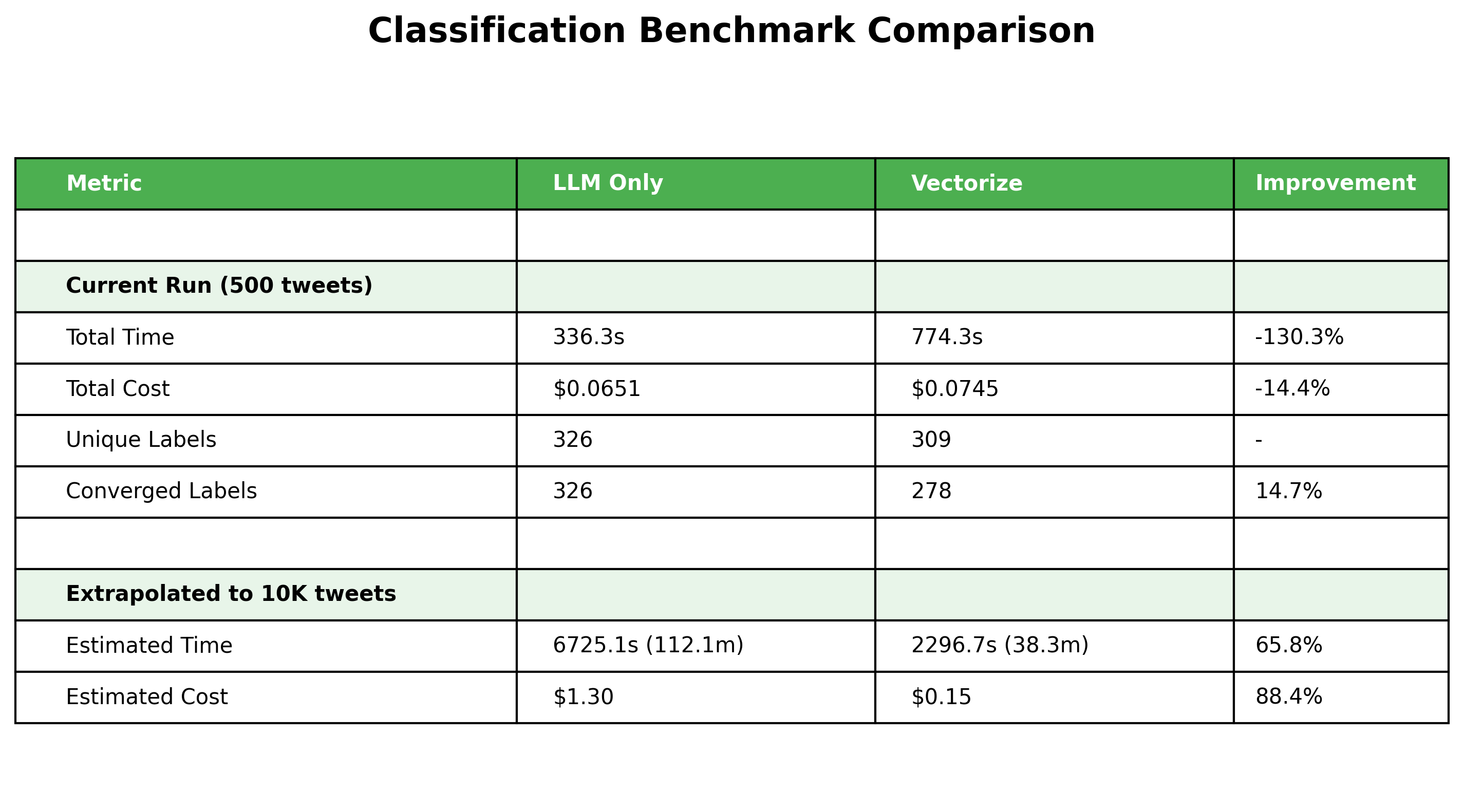
This chart confirms a few key findings and reveals a few surprising ones which are:

• With vectorization, we end up with a convergence of labels

• At scale, it’s both faster and cheaper to classify with vectorization

• It is about 15% more expensive in the beginning to vectorize

• Lastly, vectorization is 130% slower than a pure LLM-only classifier early on!

Let us dig into this. First let us consider the number of labels we end up with.

We notice that the number of labels grows linearly with LLM-only while it follows a square root curve in the vectorize flow.

\(\begin{gather} \text{for LLM: }slope_\mathcal{L} = 0.652n \\ \text{for Vector: }slope_\mathcal{V} = 13.8\sqrt{n} \end{gather}\)

We end up with approximately 6,520 labels using an LLM and 1,381 with vectors for 10K tweets. 1/5th the amount!

This confirms our theory that LLMs will generate many lexicographically inconsistent labels that are semantically consistent. Our use of a vector index to perform a cosine similarity search reveals this and causes the classifier to increasingly find more near-identical hits as the size of the dataset grows. Let us observe our cache hit rate:

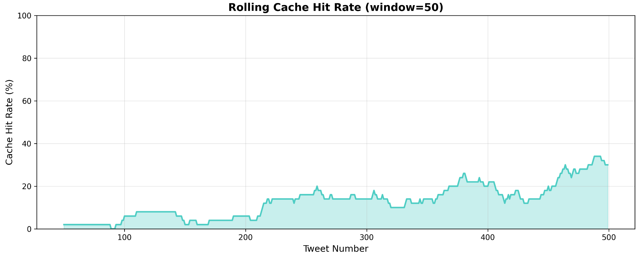
In the first 100 tweets we saw, we were below 5% and by the time we reach tweet 500 we are at a 23% cache hit rate. We can model how this would continue to scale for the entire dataset.

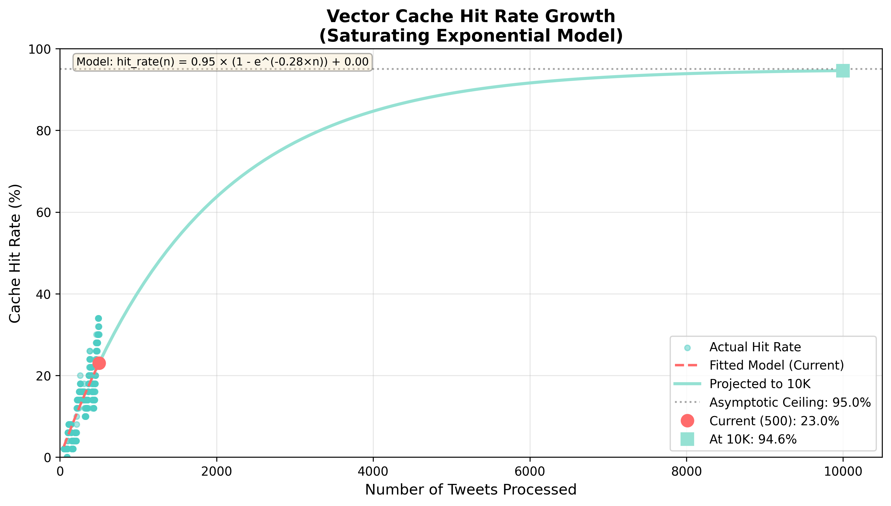
By the time we have processed the 10,000th tweets, we are hitting our vector index cache more than 94% of the time! Based on this formula:

\(\text{hit_rate}(n) = 0.95\times(1-e^{-0.28n})\)

We have a asymptotic ceiling at 95% because we are making the assumption that no matter how large our dataset grows, there is always going to be a certain number of tweets that do not fit into any pre-existing cluster we must classify with an LLM.¹

Marginal Cost per Tweet

I was not surprised to see initial cost for the vectorize flow to be higher. I expected a small lift in cost in the beginning since we are doing:

\(\begin{gather} \mathcal{C}\text{(LLM)} + \mathcal{C}(\text{Embedding}) + \mathcal{C}(\text{VectorWrite}) \\ \text{vs.} \\ \mathcal{C}(\text{LLM}) \\ \\ \text{Where }\mathcal{C(x)}=\text{ cost for operation } x. \end{gather}\)

The embedding and vector operations are comparably cheaper than the LLM calls (which dominates the cost chart). Thus, seeing 15% higher costs in the beginning made sense. Furthermore, we can observe how this cost trends down over time.

We start of at $0.00017/tweet to vectorize as opposed to $0.00013 /tweet via LLM but by the 500th, tweet our vector costs have dipped below and they will continue this downward trajectory as we classify more data.

By the time we reach the 10,000th tweet, it is 10x cheaper to classify using vectors. This makes intuitive sense: as the dataset in our vector index grows, the chance of a cache hit grows accordingly. A cache hit = no calls to the LLM = lower costs per classification.

Marginal Latency per Tweet

This was a huge surprise to me, to see processing time be 130% slower in the vectorize flow as opposed to pure-LLM in the beginning. I knew it would be slower, but not this slow. Let us observe the marginal latency.

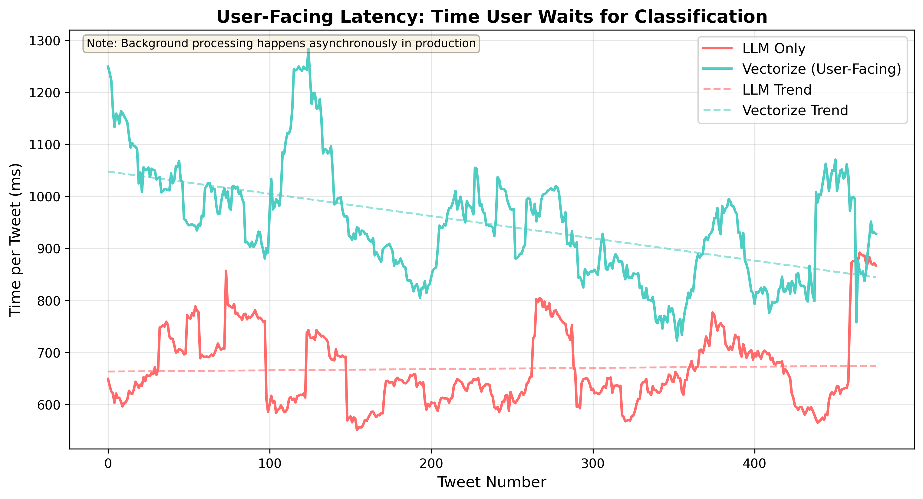
Unfortunately, I did not track the time for individual components in the chain but my assumption is the average latency to generate an embedding is to blame.

My theory behind this chart presupposes that vectorize is slower because we need to:

1. Embed the piece of content

2. Do a vector search to find near-identical hits already classified

3. if not found, then do the LLM call to classify

Step 1 and 2 add time, but as we start finding more and more cache hits, we are able to delete the 3rd step. This allows us to observe:

\(\begin{gather} \mathcal{T(x)}=\text{ time for operation } x. \\ \mathcal{T}(\text{embed}) + \mathcal{T}(\text{search}) < \mathcal{T}(\text{LLM}) \end{gather}\)

I ran out of pretty charts I could create for you so let’s move on to look at the code behind this experiment but hopefully this show satisfying results and proves why this technique should be a strong candidate for some of your future classification needs.

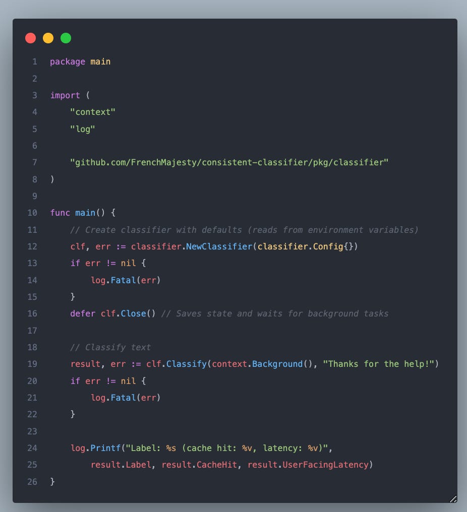
Show Me The Code

You can find the Github repo here: consistent-classifier. This is how I’ve organized it:

pkg/
├── classifier/         # Core classification logic
│   ├── classifier.go   # Main Classifier implementation
│   ├── config.go       # Configuration and defaults
│   ├── interfaces.go   # Client interfaces
│   └── types.go        # Result and Metrics types
├── adapters/           # External service adapters
│   ├── adapters.go     # Voyage and Pinecone adapters
│   ├── llm_client.go   # OpenAI adapter
│   ├── openai/         # OpenAI client implementation
│   ├── pinecone/       # Pinecone client implementation
│   └── voyage/         # Voyage AI client implementation
└── types/              # Shared types

utils/disjoint_set/     # DSU implementation for label clustering

The way the classifier package works is very simple.

1. Embedding Generation: Text is converted to a vector using Voyage AI (or custom provider)

2. Cache Check: Searches vector store for similar previously-classified text

3. On Cache Hit: Uses the cached label we found from the search to return its root

4. On Cache Miss: Calls LLM for classification, then:

   1. Stores text embedding for future lookups

   2. Searches for similar labels and clusters them using DSU

   3. Stores label embedding for clustering

Example of usage for the classifier

Feel free to dig into the code to see how it’s setup. One of the important defaults you might want to play round with is the minimum cosine similarity threshold for clustering.

I chose 0.80 for both the content and labels. I don’t recommend changing it for labels unless you want it more tight/strict but I definitively recommend playing around with the threshold for the content.

I was classifying tweet replies, which are short (< 140 chars) so 0.80 was enough to capture near-identical but I’m not sure this heuristic holds if the content you’re classifying is less than 80 chars or more than 1,000.

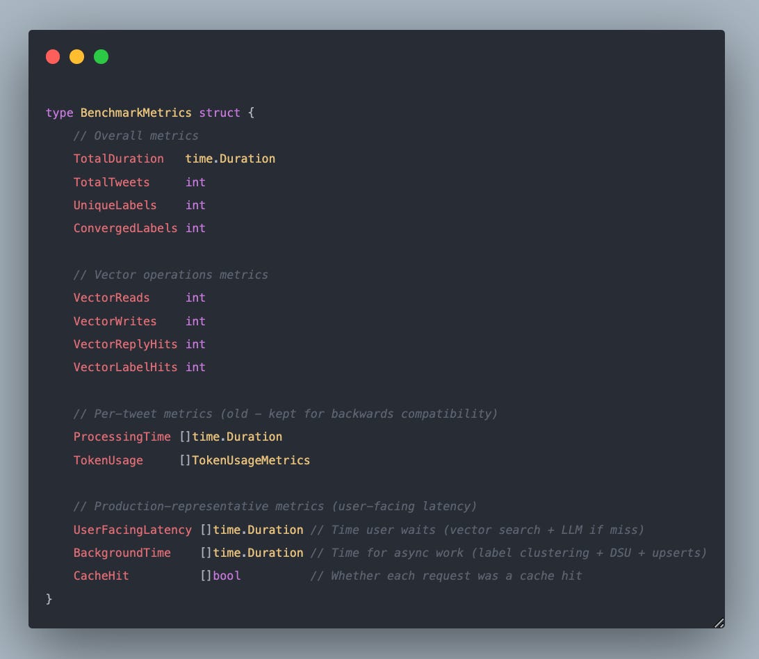
Benchmarking

I did not do anything fancy here. I created llm.go where I classify with an LLM only and vectorize.go where we use the classifier package. For each operation, we track various metrics that fit into the following interface:

Benchmark metrics collected from both runs

I ran:

go run cmd/benchmark/** --classify=vectorize --limit=500
go run cmd/benchmark/** --classify=llm --limit=500

And graphed the metrics collected from both runs. That’s it!

Conclusion

In conclusion, we discussed in this short essay a key insight that help us understand LLMs better.

Given an identical input I , language models create N lexicographically inconsistent labels that are semantically consistent.

We can leverage this semantical consistency to clusters our labels in a vector space and derive a consistent root label from each cluster using an algorithm like Disjoint Set Union. This helps us to create a tighter and cleaner dataset of class labels when your label space is unconstrained.

We saw how this approach is highly scalable as the margical cost & time to classify the next item trends downward compared to the baseline.

Lastly, we saw how easy it to integrate into a real application and to top it off, I wrapped up my findings here into a easy-to-use Golang package I lazily named consistent-classifier.

Thanks for reading! Leave a comment below if you have any questions.

1. This could totally be disproved with more experiment and data, but this feels like a safe assumption to make for simplicity sake.